The notion of a
posterior distribution comes from
Bayesian statistics. Under the Bayesian approach, prior beliefs about parameters are combined with sample information to create updated, or
posterior beliefs about the parameters. In the case of
empirical Bayes estimators, the prior information comes from the sample data as well.
Posterior distributions have found a variety of applications. A couple simple examples include:
- In student assessment student scores are often based on the posterior score distribution for the examinee. In this case, the prior distribution is often taken as the observed distribution of scores for the full sample of students, or some subset of the sample of which the individual student is a member. The sample information is given by the likelihood of the responses to test items;
- In small area estimation estimates for a small geographic area from a larger survey are often based on posterior distributions. In these cases, estimates from the whole population, or a relevant subpopulation are taken as the prior, and the (often limited) sampled cases from the target small area provide the sampled information.
The posterior information is proportional to the product of the prior information and the sample information.
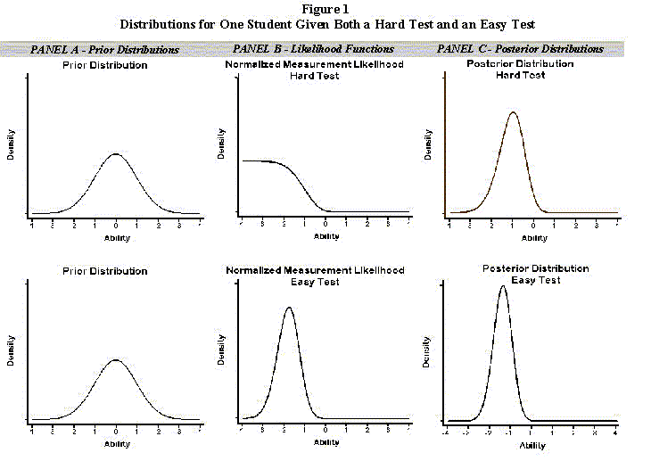
Figure 1 provides an heuristic example of how posterior distributions are formed in the case of student assessments. In that figure we present an hypothetical student with an easy form and a difficult form of the same test. The three Panels (A, B, and C) reflect the prior distribution (A) (which is the same for both tests), the measurement likelihood that constitutes the sample information (B), and posterior (C) distributions. The top row of graphs contains graphs based on the harder test, and the bottom row, the easier test. Panel A depicts the prior normal (population) distribution, which is, of course, the same regardless of the test administered. Panel B contains the measurement likelihood for our hypothetical student given the difficult (top row) and easier (bottom row) tests (both normalized to integrate to one). Notice that the likelihood given the difficult test only provides information that the student's ability is below the test's ability to measure. Taking the product of the prior and measurement distributions yields the posterior distribution.

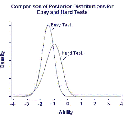
Notice that the distributions change depending on the mix of items on the test--the prior distribution is less influential when there is more information from the sample. Figure 2 overlays the two curves to facilitate comparison.

This illustration is heuristic--it presents only one possible pair of response patterns from this examinee. A more accurate representation would "average over" all possible response patterns, given their likelihood from this examinee. However, the simple example makes the relevant point.
This section provides the details of the calculation of posterior means, variances, and the standard error of the posterior means in
AM. Currently, procedures that are based on MML regression allow you to save this posterior information in the data base. The technical details follow.
Calculation of the posterior means and variance for subscales
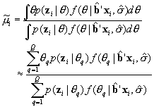
For each subscale we obtain the mean and variance for of the posterior distribution for each individual. We estimate the values using numeric quadrature on the same fixed-distance points used to estimate the MML models. Hence for any single subscale the posterior mean is estimated as

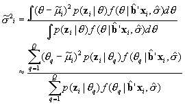
and the posterior variance is estimated as

Calculation of the moments of the posterior distribution for composite scales
The calculations of the moments of a multivariate posterior distribution most tractable when analytic results are available, as is the case for the normal distribution, and the prior distribution is multivariate normal. The measurement distribution ( ) is not. Often the measurement distributions are asymmetrical, and sometimes degenerate. Therefore, identifying the parameters of the normal distributions that provide the best approximation is not simple. This is the key problem addressed by Thomas (1993).
Here, we arrive at normal approximations by identifying the means and variances of the normal distributions that would have given rise to the estimated posteriors  and
and  . For convenience, we omit the subscript i in what follows. To arrive at this approximation let
  and
and  . Similarly, denote the moments of the prior distribution as
  and
and  . Finally, let the normal approximation to the measurement distribution have moments
  and
and  . Standard Bayesian calculations for normal distributions gives
  , where
  , and
, and  . This is all that is required to solve for the appropriate moments of the approximate multivariate normal distribution:
  and
and  .
.
To obtain the moments of the composite posterior distributions we introduce the information about the correlations among the subscales obtained from the MML composite regression. Define  where COV is the matrix formed from the estimated covariances among subscales discussed in the previous section. The approximate posterior means and variances are
  and
and  .
.
The moments of the composite posteriors are formed as  and
and 
The approximation used here works well. Appendix C presents some simple evidence demonstrating that this approximation effectively recovers variances and covariances even under extreme conditions.
Approximate standard error of the posterior mean
Formulas for the estimation of the percent of population groups above achievement levels (presented in the next section) require an estimate of the standard error around the posterior means at each observation. This appendix describes a first-order approximation of that standard error.
Our estimate of the standard error of the posterior mean begins as though the posterior distributions were approximated as normal, although in the case of subscales, they need not be. Readers should note that the posterior distributions for individual subscales are calculated on a finite set of points and may take on any shape. As described above, the composite posteriors use a normal approximation. We have found, however, that standard errors for the corresponding normal approximation work well in either case.
For this section, we change our notation slightly, and use subscripts to indicate whether parameter estimates are from the measurement (m) or prior (p) distribution. We continue to use  to indicate the mean of the posterior distribution.
Define  , where
  is the variance of the measurement distribution and
  is the variance of the empirical prior distribution. Also, note that
  where
where  represents the covariance matrix of the parameter estimates from the MML regression. Estimates of
  are themselves approximated with a first-order Taylor linearization as discussed in Binder (1983) and applied to marginal maximum likelihood estimates above and by Cohen and Jiang (1999). The specific formulas for a single subscale is given in Section 4 above, and the formula for composite scales appears in Section 5.
The normal approximation of the posterior mean would give  , where
  is the estimated empirical prior mean for examinee i, and
  is the mean of the measurement distribution for examinee i. Here, as in operational NAEP, the measurement distribution is taken as known. In what follows, we drop the subscript i to simplify the notation. We can see that
 .
.
Recognizing that  is taken as fixed, this constant drops out of the variance calculation leaving
 (4)
(4)
The third line of Equation 4 removes the constant  from variance terms, and in the final term, substitutes
  , and again drops the constant
 . The final line recognizes
In practice, we have found the last term in the final line of Equation A.1 to be typically small, generally amounting to five percent or less of the total variance, and usually substantially less. Using a first order approximation, we find that  , where
  and
and  are the measurement and empirical prior variance, respectively. Notice that the first term in this equation will tend to be small. The first term is only relatively large when the prior variance is small relative to the measurement variance. In these cases, the
  also tends to be quite small. In the interest of simplicity, we omit this term in our approximation of the variance of the mean of the posterior distribution. Hence,
Morris, C. (1983). ... Cohen, J., & Jiang T. (1998). Composite Assessment Scales and NAEP Analyses. Washington, DC: American Institutes for Research.
Thomas, N. (1993). Asymptotic corrections for multivariate posterior moments with factored likelihood functions. Journal of Computational and Graphical Statistics, 2, 309-322.
Many of the MML Regression-based procedures offer the post-hoc option of generating variables containing the posterior mean, variance, and standard error of the posterior mean. To accomplish this, right click on a icon for the completed run in the Completed Run Queue. If "posteriors" appears on an option, select it. It will automatically add these three variables to the data set. The output device (e.g., the browser) will contain a small table telling you the names of the variables created.
You probably ought to modify the label to keep a record of how the variable was created. Click here to learn about editing labels and other information.
Standard NAEP analysis is based on the evaluation of plausible values. Plausible values are random draws on the posterior distribution resulting from the the product of an empirical prior based on a composite marginal maximum likelihood regression (in which the predictors are a set of principle components from all of the data collected on the background surveys) and the measurement likelihood of the item responses.
NAEP uses a normal approximation to the posterior distribution, taking the mean and variance of the composite posterior distribution (actually, an approximation to it--see Thomas, 1993), and drawing randomly from a normal distribution with those moments.