The probit and logit models are regression models for situations in which the dependent variable is a discrete outcome, such as a “yes” or “no” decision. For example, an analyst might be interested in examining the effect of 8th grade math achievement on graduation from high school. The probit model examines the effects of a set of independent variables (Xs) on the probability of success or failure on the independent variables, P(Y). The observed occurrence of a given choice (i.e., success or failure) is taken as an indicator of an underlying, unobservable continuous variable, which may be called “propensity to choose a given alternative.” Such a variable is characterized by the existence of a threshold defining the position at which one switches from one alternative to another. For example, a student’s propensity to graduate from high school may be directly related to his or her 8th grade math achievement, which in turn may depend on family background and motivation factors. Whether a student graduates is likely to depend on whether his or her 8th grade math achievement does or does not exceed his or her threshold. This threshold, which differs across students with the same family background and motivation factors plays the role of a random disturbance.
The probit model is a probability model where:
Prob(event j occurs) = Prob(Y = j) = F[relevant effects: parameters].
Using a model of high school graduation, the respondent either graduates (Y=1) or doesn’t (Y=0) as a function of a set of factors such as parents’ education, family income, academic motivation, and so on, so that:
Prob (Y=1)=F(b'x)
Prob(Y=0)=1-F(bx)
The set of parameters b reflect the impact of changes in x on the probability. We could easily estimate this probability model as a linear regression where
y=bx+e
However, this linear probability model presents a number of problems. First, since bx+e must equal zero or one, the variance of the errors depends on b, leading to heteroscedasticity. Second, and more important, we cannot assure that the range of predictions from this model will look like probabilities since we have not constrained bx to be within the zero-one interval.
The inadequacies of the linear probability model suggest that a nonlinear specification is more appropriate. A natural candidate is an S-shaped curved bounded in the interval zero-one. One such curve is the cumulative normal distribution function corresponding to the probit model.1 This model is derived as follows. Let Y* represent an unobservable variable given by
Y*=b'x+e
where e~N(0,1) and ei and ej(i¹j) are independent. The observable binary variable Y is related to Y* in the following way:
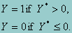
Then
E(Y) = p = P(Y = 1)
= P(Y*>0) = P(-e<b'x)
= F(b'x)
where the function F(.)represents the standard normal distribution. Thus,
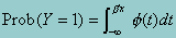
where f(t)represents the density function of t ~ N(0,1). Since p = F(b'x), we can write
F-1(p) = b'x
where F-1(p) is the inverse of the standard normal cumulative distribution function. The parameters b can be estimated by the maximum likelihood method using the log-likelihood function.
It is important to note that the parameters of the model, like those of any nonlinear regression model, will vary with the values of x. In interpreting the estimated model, it is useful to calculate this at, say, the means of the independent variables and, where necessary, other pertinent values. The formula for this robust variance estimator is as follows:
The parameter estimates  are the solution to the estimating equation
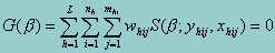
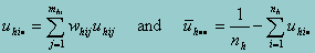
where (h,i,j) index the observations: h = 1,..., L are the strata, i = 1,..., nh are the sampled PSUs (clusters) in stratum h, and j = 1,..., mhi are the sampled observations in PSU (h,i). The outcome variable is represented by yhij, the explanatory variables are xhij (a row vector), and whij are the weights. If no weights are specified, whij = 1.
For maximum likelihood estimators, 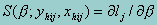 is the score vector where lj is the log-likelihood. Note that for survey data, this is not a true likelihood, but a "pseudo" likelihood.
Let
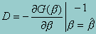
For maximum likelihood estimators, D is the traditional covariance estimate -- the negative of the inverse of the Hessian. Note that in the following the sign of D does not matter.
The robust covariance estimate is calculated by

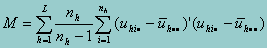
where M is computed as follows. Let uhij = S(b;yhij,xhij) be a row vector of the scores for the (h,i,j) observation. Let
Then M is given by
*******************************
1 An alternative S-shaped curve is the logistic curve corresponding to the logit model. This model is very popular because of its mathematical convenience and is given by: 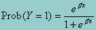 . The logistic function is used because it represents a close approximation to the cumulative normal and is easier to work with. In dichotomous situations, however, both functions are very close although the logistic function has slightly heavier tails than the cumulative normal.
Greene, W. H. (1992). Econometric Analysis, 2nd Edition. New York: Macmillan.
Kmenta, J. (1986). Elements of Econometrics, 2nd Edition. New York: Macmillan.
G. S. (1983). Limited-dependent and Qualitative Variables in Econometrics. Cambridge: Cambridge University Press.
To run Probit left-click on the Statistics menu and select Probit. The following dialogue box will open:
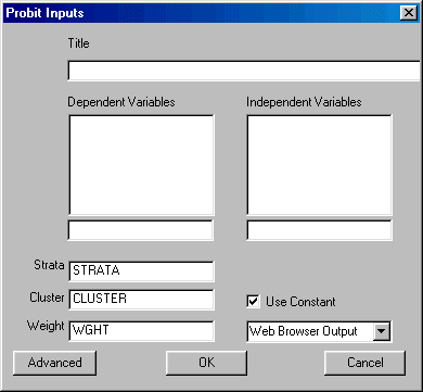
Specify the independent variables and the dependent variable. You may also elect to change the design variables, suppress the constant, and select the desired output format.
If you wish to change the default values of the program, click the Advanced button in the bottom left corner and the Advanced parameters dialogue box shown here will open:
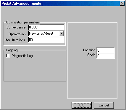
You may now edit the values for convergence, location, and scale, maximum number of iterations allowed for convergence, and change the default optimization method. You may also elect to create a diagnostic log.
When you are finished, click the OK button.
Click the OK button on the Regression dialogue box to begin the analysis.
Once the analysis is completed, you may perform t-tests on the results.