Analysts are often interested in comparing estimates of population parameter to one another, or to known constants. For example, one might test whether the observed differences in average test scores between two samples of students reflects real differences between the populations, or simple reflect chance sampling error. Evaluating questions like this typically requires an estimate of the sampling distributions of the average test scores. With the sampling distribution in hand, we can ask question of the form: "If these two populations are really the same, in what proportion of samples like this one would we observe a difference at least as large as we observed?"
Many parameter estimates are approximately normally distributed in large samples. We can use this information to construct a confidence interval around the hypothetical value of a population parameter (say, zero for an hypothesis of no difference). The probability of observing the observed difference (or a larger one) if that hypothetical value were true is given by the area under the normal curve.
As an example, suppose we observe that the average difference in test scores for two samples is 1.5, and that our sampling error (standard error) is 1. We want to know whether the true difference is greater than zero, so we ask how likely our sample would be under that condition. We can draw the normal distribution with a mean of zero (our hypothetical value) and a standard deviation of 1 (our estimated standard error). We can then mark the area above 1.5 in red, like so:
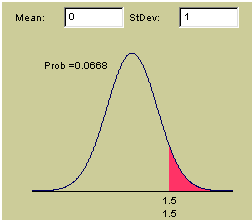
The red area marks the probability of observing a between-sample difference of the observed size or greater, if the population means were actually equal. That is 6.68% (.0668) of the are under the curve, implying that we would have about a 6.68 percent chance of observing a difference of at least this size if none really existed.
Often, analysts will not have an expectation of whether the differences will be positive or negative, so they will ask about the probability of observing an absolute difference (positive or negative) of at least that magnitude. This is called a two-tailed test, and the probability is simply twice the probability under a one-tailed test.
In smaller samples the normal approximation can prove less acceptable, and a related distribution, the Student's T distribution is used.
T-Tests comparing parameter estimates are typically conducted by forming the confidence interval around the difference ( ). Letting
  and
and  represent the sampling variances and
  represent the covariance among the estimates, the sampling error (standard error) of the difference is given by
 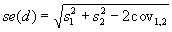 , and the T-statistic is given by
  . Typically, the null hypothesis to be tested is that no real difference exists, so the confidence intervals are formed on the basis of a distribution with a mean of zero and a standard deviation of se(d).
The degrees of freedom for the t-tests are calculated as the number of PSU less the number strata. (Strata with a single PSU contribute 1 degree of freedom--a degree of freedom is not subtracted off for the stratum). In replication procedures, the degrees of freedom equals the number of replicates that contribute to the variance estimate.
Significance testing
When conducting a t-test, analysts select a confidence level (often 95%), and declare results to be "real" if their likelihood under the null hypothesis falls below one minus the confidence level. In this case, the null hypothesis is said to be rejected.
When conducting multiple hypothesis tests, some analysts like to ensure that all of the null hypotheses for all of the "real" findings identified can be simultaneously rejected at some specified level of confidence. This is accomplished by making the confidence level more stringent via an adjustment called the Bonferroni procedure. Letting the nominal confidence level be c, the adjusted confidence level for k comparisons is given by  .
.
To access the t-test dialog, right click on an icon in the " Completed Run Queue and select "T-Tests." That will bring up a dialog much like this one:
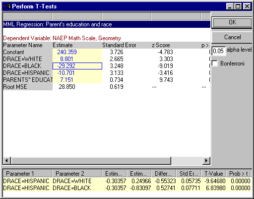
The tables is a slightly ugly version of the standard output table from the procedure. Notice that some parameter estimates are higlighted in yellow. These are available for t-testing. To conduct a t-test:
- Move the cursor over the first item in the comparison. The cursor will turn into a hand.
- Click on the highlighted item. A blue outline should appear around that cell. This is now the "anchored parameter." Any other cells you click on will be compared to the outlined cell
- Move the cursor over the parameter to be compared--again, it should turn into a hand.
- Click on the cell to be compared. The results of the t-test will appear in the window at the bottom of the dialog box. Significant results will be higlighted in yellow.
- To un-anchor the anchored parmeter (to conduct tests not invovling that parameter), simply click on the anchored parameter.
- When you have completed your t-tests, press the "OK" button and the results will be sent to your output browser.
To use a Bonferroni adjustment, select the check box labeled "Bonferroni."