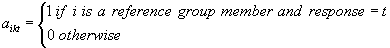
This procedure is widely used to evaluate differential item function (DIF). Psychometricians use measures of DIF to identify items that may exhibit biases for or against identifiable groups in the population (e.g., male or female, black or white, etc.).DIF measures typically compare the performance similarly proficient members of different groups on a particular target item. If the performance of similarly proficient students differs across groups, the item is said to exhibit “differential item function.”
In virtually all educational testing programs, DIF statistics are calculated as though they come from a simple random sample (SRS) from the population. In fact, virtually no educational testing programs select simple random samples—schools are usually sampled from within districts, and whole classrooms of students are tested together. Often these selections are made with unequal probabilities, used to ensure adequate representation of members of minority groups.
Complex sample designs violate the assumptions on which the simple random sample test statistics are based.For example, most statistics assume that all selected units are sampled independently. In a clustered design (where, for example, schools are selected then students within the selected schools participate), the selection of a higher level unit (e.g., school) determines the selection of subsequent sampling units (e.g., students). Because students within a school tend to have more in common with each other than with a student selected at random from the whole population, the clusters (schools) exhibit less variation than the population at large. Essentially, each student sampled from the same school adds less new information to the sample than would a student selected at random from the whole population.SRS formulas for standard errors and test statistics therefore tend to over-estimate significance levels (e.g., Kish, 1965; Sarndal, Swenssen and Wretman, 1992).
By ignoring the complex sample design, typical DIF statistics overstate the proportion of items flagged for further evaluation. The evaluation usually involves review by a fairness committee. While over-flagging items may seem a conservative strategy, in practice it may not be. Human committees must individually analyze each flagged item. Spurious flags take time and attention away from items that are more likely to really function differently. Furthermore, committees become accustomed to seeing items that are flagged as exhibiting DIF, but do not seem unfair to any group. This may lead them to more quickly accept items as fair with fewer second thoughts.<
This paper presents a method for analyzing DIF that appropriately accounts for the complex sample designs found in most assessment databases. While many different statistics are used to indicate DIF, we focus on a generalized version of the Mantel-Haenzel (MH) Chi-Square DIF statistic (Mantel and Haenzel, 1959), which is the indicator most often used in applied testing programs. The original MH statistic applies only to binary items, while the generalized Mantel-Haenzel (GMH) statistic extends the approach to polytomous items (Somes, 1986).
In the dichotomous case, the data can be summarized as in Exhibit 1. Typically, the majority group is referred to as the reference group , and DIF analyses evaluate whether the item functions differently for the focal group.
Exhibit 1: Response classification table for an item
|
|
Reference Group (R)
|
Focal Group (F)
|
Total
|
|
Correct Response
|
a
|
b
|

|
|
Incorrect Response
|
c
|
d
|

|
|
Total
|

|

|
T
|
The cells of the table would include the count (or estimated population total) of people falling in the cell.For example cell a would include an estimate of the total number of reference-group members who answered the item correctly.
The standard MH DIF procedure begins by stratifying the sample of examinees based on some measure of proficiency. This yields a set of 2x2 tables similar to Exhibit 1.Typically, this measure is a score based on the items on the test. In what follows, we index the elements of Exhibit 1 with k for k={1,2…,K} strata.
The MH chi-square statistic is calculated as,
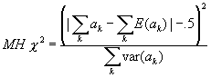 (1)
(1)
The -.5 in the numerator is a small continuity correction which is ignorable except in very small samples. The expectation  is given by
 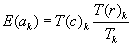 , which is the number of correct responses from the reference group if both groups responded correctly in exactly the same proportion (within stratum k).
Looking at Equation 1, we can see why this estimator might be particularly sensitive to a clustered sample.Within each population subgroup, the data are carved up into relatively homogenous strata based on student performance. An item on a topic covered recently (or not covered yet) in that school could show substantially differences in performance across schools. In samples of reasonable size, many or all of the focal group members in a particular stratum may be drawn from the same school or classroom, confounding school differences with group differences. The result could be an overestimate of DIF. Appropriately accounting for the sample design alleviates this problem.
The GMH statistic generalizes the MH statistic to polytomous items (Somes, 1986).
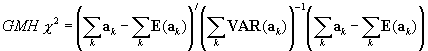
where  is a t-1x1vector of responses, corresponding to theT response categories of a polytomous item (excluding one response). Each element reflects the number of reference group responses in that category. The
  are calculated analogously to the corresponding elements in Equation 1, and
  is a t-1 x t-1variance matrix for stratumk.
Under simple random sample assumptions, the elements in the cells are simply counts, and the variances are calculated directly from the sample sizes. The next section describes the procedures that estimate the GMH  in complex samples.
GMH  for Complex Samples
This section defines a GMH estimator for samples collected according to an unequal-probability, stratified, clustered design, or designs that can be reasonably approximated as such.
We define the sampling weight as  , where
  is the probability of selection. We index the sampling strata with h = {1,2,…,H} , and caution the reader not to confuse the sampling strata with the stratification based on proficiency groupings in the calculation of the GMH statistic.Finally, we index primary sampling units within sampling strata with
  .
.
We begin with by calculating estimates of the elements of  , which are estimated by
and  .
.
Calculation of the focal group totals follows immediately by replacing the group membership condition.With these in hand, calculation of the expectations can use the same formulas presented above.
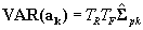
Calculation of  is a bit more complicated. The usual estimator assumes that the strata defined by the matching variables are independent (which we also assume, with caution because the clustering can violate this assumption), and that the marginal totals in each stratum are known constants rather than random variables.The latter assumption is sensible because we are not interested in estimating how the population divide into these strata—only in how groups in the population perform on the assessment, given that they fall into the stratum (recall here that we are talking about the strata defined by the matching variable, rather than the sampling strata).
Under the null hypothesis in a simple random sample for the dichotomous MH statistic,  , where
  is the proportion of correct responses in stratum k . We recognize the term
  as the sampling variance of
  under a simple random sample. In the polytomous case, the final term becomes
 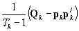 , where
  is a diagonal matrix with
  , the proportion responding in category tfort={1,2,…,t-1} on the diagonal, and
  is a tx1 vector containing the
  . We can rewrite this estimator generically (for the complex or simple sample) as
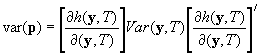
where  is the estimate of the sampling variance matrix of the estimate of
To adapt this to a complex sample, we use a Taylor-series expansion. We begin by calculating a design-consistent (i.e., appropriate for the sample design) variance matrix for the total number of examinees responding in each response category within each stratum (that is, the strata defined by the matching variable). We do this rather than calculate the entire, cross-strata variance matrix in the interest of computing time—the matrices can grow quite large.The between-strata variances should be negligible. The design-consistent estimates of the sampling variance of the population totals (  )
)
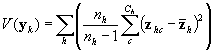
where  ,
,  is a vector of ones and zeros indicating examinee i ’s response category.
  is the average cluster total within stratum h . Essentially, the variance is the weighted stratified estimator of the between-cluster variance.
With the variance estimates for the population totals in hand, we can calculate estimates of the sampling variance of the proportions. Note that the proportions may be considered ratios of two population totals--the total for the cell in the numerator, and the total for the row (the sum of the cells) in the denominator. We can specify the ratio as the solution to the following estimating equation involving population totals (we omit the index for matching-strata, k in what follows because all formulas apply to an individual stratum):
where N is the estimate of the Using the first-order Taylor-series estimate of the variance of estimates from this estimating equation, we have
 .
.
The variance of the estimated row total (T), along with its covariances with the frequency estimates, can be calculated as a linear combination of the  . We begin by augmenting var(y) with an extra row and column for N. To do so, define the t-1 x t design matrix D, which has the following form:
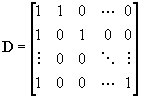 .
.
The augmented variance matrix is given by
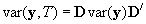 .
.
The derivative matrix for t-1 proportion estimates from t parameter estimates takes a similar form, where
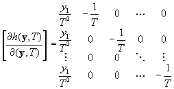
The resulting matrix estimates the sampling variance of the estimated proportions (  ).
).
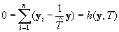
The test statistic
The chi-square statistic is appropriate for large samples. In a complex sample the variance is often estimated from a small number of PSUs, an F-statistic is usually more appropriate. AM transforms the chi-square (call it Q>) to a variable with an approximate F distribution:
F=Q/(K-1)
The degrees of freedom are given by the number of PSUs less the number of strata.
[1]Stratification can offset some of this effect, but appropriate complex sample standard errors quite unlikely to match SRS formulas serendipitously.
[2] The particular statistics used to indicate DIF vary in the way they identify “similarly proficient” examinees, the way they compute a difference in performance, and they way they aggregate across sets of sets of similarly proficient students to obtain an estimate for the whole population. Holland and Wainer (1992) provides a good overview of the variety of methods available.
[3]
Holland and Thayer (1988) and Donoghue, Holland and Thayer (1994) present arguments in favor of including the target item in the measure used for matching. The empirical evidence in the second article suggests this strategy reduces the MH prodedure’s often-noted overidentification of DIF. The details of the matching procedures are tangential to the central issue discussed here.
[4] In fact, this formula overlooks possible covariances between the strata defined by the matching variables. Clustered sampling can induce these correlations. The formulas presented here assume that these covariances are small enough to be ignorable, though the issue is probably worthy of further investigation.
Holland, W. P. & Thayer, D. T. (1988). Differential item performance and the Mantel_Haenszel procedure. In H. Wainer & H. I. Braun (Eds.), Test validity (pp. 129-145). Hillsdale, NJ: LEA.
Holland, P.W., & Thayer, D.T. (1986) Differential item performance and the Mantel-Haenszel procedure (Technical Report No. 86-69). Princeton, NJ: Educational Testing Service.
Holland, P. W., & Wainer, H. (Eds.). (1992). Differential itemf unctioning: Theory and practice . Hillsdale : Lawrence Erlbaum Associates, 1992.
Kish, L. (1965). Survey Sampling. New York: John Wiley and Sons.
Mantel, N., & Haenszel, W. (1959). Statistical aspects of the analysis of data from retrospective studies of disease. Journal of the National Cancer Institute , 22:719-748.
Masters, G.N. (1982).A Rasch model for partial credit scoring. Psychomotrika, 47, 149-174.
Rasch, G. (1960). Probabilistic models for some intelligence and attainment tests . Chicago: The University of Chicago Press.
Särndal, C. E., Swensson, B., & Wretman, J. (1992). Model Assisted Survey Sampling . New York: Springer-Verlag.
Somes, G. W. (1986). The generalized Mantel Haenszel statistic. The American Statistician, 40:106-108.
Wright, B.D., and Stone, M.A. (1979). Best Test Design. Chicago: MESA Press.
Zwick R., Thayer D.T. (1996) Evaluating the magnitude of Differential Item Functioning in polytomous items. Journal of Educational Statistics , 21:3, 187-201.