Regression

The goal of regression analysis is to determine how and to what extent the variability of the dependent variable depends upon the variability in one or more independent variables. For example we might want to determine the effect of hours of study, X, on math achievement, Y. Because performance on Y is likely to be affected by factors other than X as well as by random error, it is unlikely that all individuals who study the same number of hours exhibit identical math achievement. But if X does affect Y, the means of the Y’s at different levels of X would be expected to differ from each other. When the Y means for the different levels of X differ from each other and lie on a straight line, this is what we call a linear regression of Y on X. This idea can be expressed by the following linear model:

Y_i=a+bX+e_i

where Y_i is the score of individual i; a is the mean of the population when the value of X is zero, and is referred as the intercept; b is the regression coefficient in the population, indicating the slope of the regression line; and e_i is a random error term for individual i. The regression coefficient, b indicates the effect of the independent variables on the dependent variable. Specifically, it indicates the change in Y for each unit change of X. It can be seen from the above equation that each person’s score, Y_i, is composed of two parts: a fixed part common to all individuals, indicated by a+bX; and a random part, e_i, unique to each individual.

The above equation was expressed in terms of population parameters. For a sample it is written as:

Y=a+bX+e

where a is an estimator of a, b is an estimator of b, and e is an estimator of e_i.

In an ideal situation, the goal of the researcher would be to explain Y, math achievement on the basis of X, hours of study, without any error. However it is unlikely that students studying the same number of hours will all have identical math achievement. Other variables not included in the model (e.g., motivation, past math experience) as well as errors in the measurement of the variables will lead to variability in students’ performance. The sources of variability in Y not due to X are all subsumed under the error term, e. Thus, e becomes the part of the dependent variable, Y, that is not explained by X.

The goal of regression analysis is to find a solution for the constants a and b so that e, the errors committed in using X to predict Y are minimized. However, because positive errors will cancel negative ones and the sum of errors will always be zero, instead it is the sum of the squared errors (Se²) that is minimized. This is what is called a least squares solution.

The above example was limited to simple regression analysis with only one <independent variables. In most cases, however, analysts are interested in assessing the effects of multiple independent variables on a dependent variable. The principles of simple linear regression are easily extended to multiple regression to accommodate any number of independent variables as the following equation indicates:

y=a+b₁+X_i+b₂X₂+...+b_kX_k+e

where b₁,b₂,...,b_k are regression coefficients associated with the independent variables X_i,X₂,...,X_k. As was the case in simple linear regression, a least square solution that maximizes the sum of squared errors is sought. The major difference is that with more than one independent variables, solving for the b’s in the above equation is considerably more difficult. In particular, in multiple regression, solving for the b’s involves taking the correlation of the multiple predictor variables into account to eliminate potentially redundant information (i.e., the amount of variance that these variables have in common). Therefore, to calculate the part of Y that is determined by say, X₁ and X₂, it is necessary to subtract the amount of variance these two variables have in common so that it will not be counted twice.

Because data obtained from complex surveys typically violate the assumption of independence of observations (when for example students are sampled in entire classrooms) necessary to obtain unbiased estimators, estimation routines must take the feature of the sample statistics. The regression procedure uses a robust variance estimator known as a weighted first-order Taylor-series linearization method (Binder, 1983) that corrects for heteroscedasticity (i.e., different error variance) as a result of stratified cluster sampling.The formula for this robust variance estimator is as follows:

The parameter estimates are the solution to the estimating equation

where (h,i,j) index the observations: h = 1,..., L are the strata, i = 1,..., n_h are the sampled PSUs (clusters) in stratum h, and j = 1,..., m_hi are the sampled observations in PSU (h,i). The outcome variable is represented by y_hij, the explanatory variables are x_hij (a row vector), and w_hij are the weights. If no weights are specified, w_hij = 1.

For maximum likelihood estimators, is the score vector where l_j is the log-likelihood. Note that for survey data, this is not a true likelihood, but a "pseudo" likelihood.

Let

For maximum likelihood estimator, D is the traditional covariance estimate -- the negative of the inverse of the Hessian. Note that in the following the sign of D does not matter.

The robust covariance estimate is calculated by

where M is computed as follows. Let u_hij = S(b;y_hij,x_hij) be a row vector of the scores for the (h,i,j) observation. Let

Then M is given by

*******************************

¹ An alternative S-shaped curve is the logistic curve corresponding to the logit model. This model is very popular because of its mathematical convenience and is given by: . The logistic function is used because it represents a close approximation to the cumulative normal and is easier to work with. In dichotomous situations, however, both functions are very close although the logistic function has slightly heavier tails than the cumulative normal.

Binder, D. A. (1983). On the variances of asymptotically normal estimators from complex surveys. International Statistical Review, 51, 279-292.

Greene, W. H. (1992). Econometric Analysis, 2nd Edition. New York: Macmillan.

Pedhazur, E. J. (1982). Multiple Regression in Behavioral Research, 2nd Edition. Fort Worth, TX: Harcourt Brace Jovanovich.

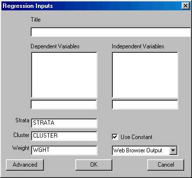
To run Regression left-click on the Statistics menu and select Regression. The following dialogue box will open:

Specify the independent variables and the dependent variable. You may also elect to change the design variables, suppress the constant, and select the desired output format.

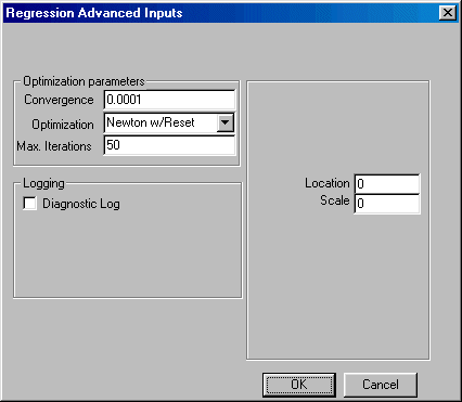
If you wish to change the default values of the program, click the Advanced button in the bottom left corner and the Advanced parameters dialogue box shown here will open:

You may now edit the values for convergence, location, and scale, maximum number of iterations allowed for convergence, and change the default optimization method. You may also elect to create a diagnostic log.

When you are finished, click the OK button.

Click the OK button on the Regression dialogue box to begin the analysis.

Once the analysis is completed, you may perform t-tests on the results.