The idea behind maximum likelihood (ML) estimation is to identify population parameters (e.g., mean, variance) that are most likely to have generated the observations in the sample data. This is done iteratively by trying various arbitrary values of the population parameters until we identify these values that maximize the joint likelihood of obtaining the sample observations.
The principles of Maximum Likelihood (ML) were developed by Fisher (1950) as a tool to assess the information contained in sample data. We must start by assuming the general form of the population distribution from which a sample is drawn. Typically, one would assume a normal distribution but ML does not restrict one to this assumption. Even by assuming that we know the general form of the distribution, we still do not know the population parameters that give this distribution its specific functional form. The idea of ML is to choose arbitrary values of these population parameters and ask what is the likelihood that these arbitrary parameters yield the observed data in the sample. When we have more than one observation on a given random variable-typically the case in social science analysis-then we are concerned with the joint likelihood of obtaining a sample of observations. Specifically, ML estimation tries a succession of arbitrary population parameters values until it identifies the ones that make the sample observations have the greatest joint likelihood. The values of the population parameters that maximize the joint likelihood are called the maximum likelihood estimators (MLE) of the population parameters.
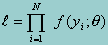
Obtaining the maximum likelihood estimators involves specifying the likelihood function (the formula specifying the joint probability distribution of the sample) and finding those values of the parameters that give this function its maximum value. In other words, given a sample of observations y, find a solution for the parameter(s) q that maximizes the joint probability function f(y;q). Because observations on y are assumed independent of one another, the joint probability distribution can be written as the product of the individual marginal distributions. We then maximize the likelihood function:
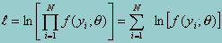
Because products are computationally difficult to work with, one generally works with the logarithm of the above likelihood functionsince logs can be summed over observations. Furthermore, since a log transformation is a monotonic transformation (i.e., whenever l is increasing, its logarithm is also increasing) the point corresponding to the maximum of l is also the point corresponding to the maximum of the log of l. Hence, to obtain the MLE, one typically works with the log of the above formula:
The solution for q that maximizes the log likelihood function in the above equation is called the Maximum Likelihood estimator (MLE). To find the MLE, we take the first derivative of the above function with respect to q, set it to zero, and solve for q. The first derivative represents the slope of the lines tangent to the log-likelihood. By setting it to zero, we establish the necessary condition for a function to be at its maximum (or minimum) by forcing the slope of the tangent to also be zero and thus a horizontal line (Kmenta, 1986).To make sure that the solution gives indeed the maximum value of l (rather that its minimum), we check the second derivative. If the second derivative is less than zero, then the curve is concave down and the solution is a maximum. When there is more than one unknown parameter in the likelihood function, solving for q involves working with partial derivatives instead.
Eliason, S. R. (1993) Maximum Likelihood Estimation: Logic and Practice. Sage University Paper 96: Quantitative Applications in the Social Sciences.
Fisher, R. A. (1950). Contributions to Mathematical Statistics. New York: Wiley.
Kmenta, J. (1986). Elements of Econometrics, 2nd Edition. New York: Macmillan.
NAEP results are estimated through models that rely on Marginal Maximum Likelihood (MML) estimation procedures. These MML procedures are themselves extensions of the principles guiding Maximum Likelihood (ML) estimation for cases when the variables of interest (e.g., proficiency) are only partially observed.