This specialized procedure provides marginal maximum likelihood estimates of the average of a latent trait (e.g., proficiency in a subject) within groups defined by an nominal variable (e.g., age groups, income groups). Typically, analysis of large scale assessments proceeds in two steps. First, the parameters of the measurement model are estimated from a large sample and taken as known in the second step. The second step estimates the proficiency distribution within groups via marginal maximum likelihood according to a specified model.
The MML nominal tables procedure arises in response to the incompatible assumptions typically required at the two stages of analysis. The first step often involves a measurement model that assumes a normal population distribution. Typical analytical methods used in the second step often estimate group means as the means of normal distributions within groups (such analysis may be accomplished via an MML regression with dummy variables indicating group membership as predictors). But if the subgroup distributions are normal, then the population distribution must be a finite mixture of normal distribution, and hence not normal. This incompatibility can lead to inconsistent estimates. The MML ordinal tables procedure maintains the common first-step assumption that the target trait is normally distributed in the population.
The MML nominal tables procedure was developed to consistently estimate subpopulation distributions when the groups are defined by values of a nominal variable (e.g., race, gender, region). The general approach to estimation assumes that the nominal variable reflects the interplay among several continuous variables (say x1*, x2* and x3*). However, rather than directly observe any of these variables, all we know through the observed variable (say x) is which of the latent variables assumes the highest value. Thus, for example, x = 1 if x1* > x2* and x1* > x3*. This general approach is similar to that typically taken in a multinomial logit context (McFadden, 1973). We can estimate the parameters of the joint distribution (q,x*) along with the parameters defining the relationship between x (the nominal variable) and x*. With these estimates in hand, we can infer the distribution of q within groups while retaining the assumption of a normal subpopulation distribution.
Let q represent an inherently unobservable latent variable, which is imperfectly measured by a series of items z (e.g., test questions, survey items). Also, assume the relationship between the measured items and the underlying latent variable is known. Typically, in large-scale assessments, the items are given to a large enough sample that the parameters of the model specifying the relationship between items and underlying traits are estimated with sufficient precision to ignore this uncertainty in the relationship (Mislevy 1985, 1991). Also, let x represent a nominal variable defining the groups to be compared. The normal distribution of q is given a priori, but the conditional distribution (q|x) remains unknown.
Suppose, however, that x represents a partial observation on several normal variates x* , such that x = k if xj* < xk* for all  for groups j = {1,2,...,m). This sort of formulation is quite natural in many situations, for example, a survey’s respondents might classify themselves in the race group with which they most identify. Further, assume that the relationship between q and each x* is linear, which may not be true but is a common and powerful approximation. (Even without the latent trait justification for the model, the probability model developed below remains reasonable and tractable. Below, we will also assume that, conditional on q, the x* are independent of one another.)
With this setup, we can write

where aj and bj are the parameters to be estimated, and uj is a normally distributed residual. Letting rj represent the correlation between q and xj*, this formulation yields xj*|q~N(aj + bjq,1), so that rj = bjsq / sxj*. Since the means and variances of the latent variables x* are arbitrary, r (along with the parameters of the q distribution) provide sufficient statistics for the multivariate normal distribution (q,x1*,x2*,...,xm*), from which we will infer the values of the table cells.
This model maintains an indeterminacy of scale and location. Without loss of generality, this indeterminacy is resolved by fixing a1 = b1 = 0 and var(uj) = 1 for all j. In theory, we need not constrain the uj to be independent of one another; however, estimation when they are correlated requires multidimensional integration that increases with the number of categories. While this is tractable up to three or four categories, the estimation becomes too burdensome beyond this (Greene 1990, p. 703). Therefore, we assume a variance and covariance matrix that is diag(1,1,1,...,1), which resolves the indeterminacy of scale by fixing the variances. We note that this assumption of conditional independence is analogous to that made in the well-known multinomial logit model (McFadden 1973).
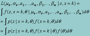
For an observation falling in the group x = k, the likelihood function is given by

Suppressing the dependence on the parameters in the right-hand side, and drawing on the definition of conditional density and then the standard IRT assumption of conditional independence, we obtain

Replacing  <
<
Using the conditional independence of x1*, x2*,...,xm*, we further obtain

The conditional distribution of xj* given q is normal with mean aj + bjq and unit variance, so p(xj < xk|q) = F(xk - aj - bjq), where F(.) is the standard normal distribution function. The distribution of q is also normal a priori, generally with known mean and variance, though these parameters may also be estimated (which may provide a useful approximation when a subset of the data is analyzed). Also, p(z|q) is a known function of the data (generally not normal) and may be directly calculated. Note that the likelihood requires only a double integral regardless of the number of groups involved.
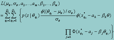
Given the unpredictable form typically taken by p(z|q), it is prudent to approximate the double integrals over a finite number of points. Thus, defining Q1xQ2 quadrature points corresponding to q and xk*, we can write the likelihood function.

where F is the standard normal density function. Taking logs and summing over the sample observation yields the log-likelihood for the sample data.
The estimates can be used to construct “implicit tables”, that is the predicted table that would result from the observed sample. The simplest way to do this entails estimating the densities qq1|x = k. Based on the density estimate, one can calculate the mean and variance within group k (see Cohen & Jiang, 1999).
Cohen, J., & Jiang, T. (1999). Comparison of Partially Measured Latent Traits Across Nominal Subgroups. Washington, DC: American Institutes for Research.
Greene, W. H. (1993). Econometric Analysis, 2nd Edition. New York: Macmillan.
Mislevy, R. J. (1985). Estimation of latent group effects. Journal of the American Statistical Association, 80, 993-997.
Mislevy, R. J. (1991). Randomization-based inference about latent variables from complex samples. Psychometrika, 56, 177-196.
McFadden, D. (1973). Conditional logit analysis of qualitative choice behavior. In P. Zarembka (Ed.), Frontiers in Econometrics. New York: Academic Press.
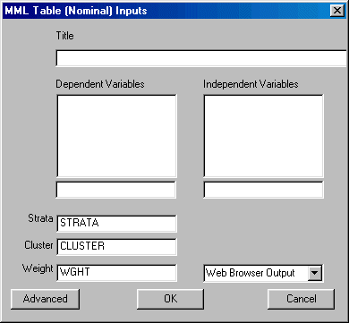
run MML Nominal Table left-click on the Statistics menu and select "MML Table (Nominal)." The following dialogue box will open:

Specify the independent variable and the dependent variable. There are several specific requirements for variables when running the MML Nominal Table. Users may select a single categorical independent variable. The model is somewhat more general than the ordinal version, and can accommodate ordinal or nominal classification variables; however, for ordinal variable the ordinal model is more efficient.
The dependent variable for this analysis is a univariate assessment scale; that is, a single subtest of a single test. The user must select a test from the Test box, and a subtest from the Subtest box. You may also elect to change the and design variables and select the desired output format.
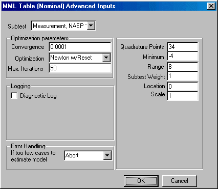
If you wish to change the default values of the program, click the Advanced button in the bottom left corner and the Advanced parameters dialogue box shown here will open:

You may now edit the values for quadrature points, minimum, range, subtest weight, convergence, maximum number of iterations allowed for convergence, and change the default optimization method. You may elect to create a diagnostic log and indicate whether you would prefer the program to abort the analysis or issue a warning when the data contains too few cases per cell to estimate the model.
When you are finished, click the OK button.
Click the OK button on the MML Table (Ordinal) dialogue box to begin the analysis.
Once the analysis is completed, you may perform an underlying table or variance covariance matrix