This specialized procedure provides marginal maximum likelihood estimates of the average of a latent trait (e.g., proficiency in a subject) within groups defined by an ordinal variable (e.g., age groups, income groups). Typically, analysis of large scale assessments proceeds in two steps. First, the parameters of the measurement model are estimated from a large sample and taken as known in the second step. The second step estimates the proficiency distribution within groups via marginal maximum likelihood according to a specified model.
MML ordinal tables procedure arises in response to the incompatible assumptions typically required at the two stages of analysis. The first step often involves a measurement model that assumes a normal population distribution. Typical analytical methods used in the second step often estimate group means as the means of normal distributions within groups (such analysis may be accomplished via an MML regression with dummy variables indicating group membership as predictors). But if the subgroup distributions are normal, then the population distribution must be a finite mixture of normal distribution, and hence not normal. This incompatibility can lead to inconsistent estimates. The MML ordinal tables procedure maintains the common first-step assumption that the target trait is normally distributed in the population.
The MML ordinal tables procedure was developed to consistently estimate subpopulation distributions when the groups are defined by values of an ordinal variable (e.g., age groups, income groups). The general approach to estimation assumes that the ordinal variable represents a partial observation on an underlying continuous distribution (say x*). Thus, rather than directly observe values of x*, we observe only that it falls within some range (e.g., if x* represents age, then we observe x, which might take on a few categories such as 16-24, 25-34, etc.). We can estimate the parameters of the joint distribution (q,x*) along with the parameters defining the relationship between x (the ordinal variable) and x*. With these estimates in hand, we can infer the distribution of q within groups while retaining the assumption of a normal population distribution.
Let q represent an unobservable latent variable, which is imperfectly measured by a series of items z (e.g, test items). Also assume that the relationship between the measured items and the underlying latent variable is known, letting x represent an ordinal variable defining the groups to be compared. Typically, in large scale assessment, the items are given to a large enough sample that the parameters of the model specifying the relationship between items and underlying traits are estimated with sufficient precision to ignore this uncertainty in the relationship (Mislevy, 1985; 1991). The normal distribution of q is given a priori, but the conditional distribution q|x) remains unknown. However, since x is ordinal, we can assume that x is a partially observed realization of the standard normal variate x*, such that

and that the relationship between x* and q is linear. This assumption is analogous to that made in the ordered probit model (Zavoira & McElvey, 1975).
The likelihood function is given by,

Suppressing the dependence of the parameters on the right-hand side and employing the standard IRT assumption of conditional independence, we can write

Recall that the probability of the item responses given q, (p(z|q)) is assumed known. Again invoking the definition of a conditional density, and replacing the observed x with the integral of x* over the range that would yield the observed value of x, yields

The conditional distribution f2 of these two normal distributions is also normal, with mean  and variance 1 - r2, where r is the correlation between q and x*.
The parameters of the distribution f1 can also be estimated. Also, p(z|q) is a known function of the data (generally not normal) and may be directly calculated.
Given the unpredictable form typically taken by p(z|q), it is prudent to approximate the outer integral over a finite number of points. Thus, defining Q quadrature points, we can write the likelihood function as,

Where F(x) is the standard normal cumulative distribution function. Taking logs and summing over the sample observation yields the log likelihood for the sample data.
This model yields estimates of the mean and variance of the proficiency distribution, the correlation between that distribution and the underlying distribution of x*, and the estimated thresholds along x* that correspond to cut points between the levels of x. These estimates can be used to construct “implicit tables,” that is, the predicted table that would result from the observed bivariate relationships. The simplest way to do this entails calculating the mean and variance of the (possibly doubly) truncated normal distribution within each cell, given the estimated mean, variance, correlation, and thresholds (see Maddala, 1983 p. 369-370).
Tests of the significance of relationships apparent in the tables reduce to tests of the parameters of the original model. For example, a test of whether the cell means differ reduces to a test of whether the correlation parameter is significant and whether the difference between the threshold values is significant.
Cohen, J. (1998). Subgroup Comparisons of Partially Measured Latent Traits. Washington, DC: American Institutes for Research.
Maddala, G. S. (1983). Limited-dependent and Qualitative Variables in Econometrics. Cambridge: Cambridge University Press.
Mislevy, R. J. (1985). Estimation of latent group effects. Journal of the American Statistical Association, 80, 993-997.
Mislevy, R. J. (1991). Randomization-based inference about latent variables from complex samples. Psychometrika, 56, 177-196.
Zavoira, T., & McElvey, W. (1975). A statistical model for the analysis of ordinal level dependent variables. Journal of Mathematical Sociology, Summer 1975, 103-120.
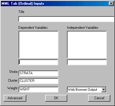
To run MML Ordinal Table left-click on the Statistics menu and select "MML Table (Ordinal)." The following dialogue box will open:

Specify the independent variable and the dependent variable. There are several specific requirements for variables when running the MML Ordinal Table. Only a single independent variables can be selected from the independent variables list. It is the user’s responsibility to select an ordinal or binary independent variables if they are using this model.
The dependent variable for this analysis is a univariate assessment scale; that is, a single subtest of a single test. The user must select a test from the Test box, and a subtest from the Subtest box. You may also elect to change the starting values and design variables and select the desired output format.
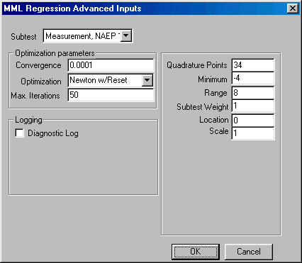
If you wish to change the default values of the program, click the Advanced button in the bottom left corner and the Advanced parameters dialogue box shown here will open:

You may now edit the values for quadrature points, minimum, range, subtest weight, convergence, maximum number of iterations allowed for convergence, and change the default optimization method. You may elect to create a diagnostic log and indicate whether you would prefer the program to abort the analysis or issue a warning when the data contains too few cases per cell to estimate the model.
When you are finished, click the OK button.
Click the OK button on the MML Table (Ordinal) dialogue box to begin the analysis.
Once the analysis is completed, you may perform an underlying table or variance covariance matrix