The MML Regression procedure estimates a linear regression in situations where the dependent variable (e.g., proficiency on a subtest) is only partially observed. In such cases, we observe a pattern of responses to items rather than observing proficiency directly. Hence, an individual’s score is represented by a probability distribution over all possible scores instead of a single value for the dependent variable. Parameter estimates are obtained through marginal maximum likelihood.
As in classical linear regression, the dependent variable (e.g., proficiency, denoted q) in MML regression is modeled as a linear combination of independent variables and a normally distributed error term:
qi = a + b1X1 + b2X2 + ... + bkXk + ei
or in matrix notation:

However, unlike in classical linear regression, since proficiency (qi) is only indirectly observed through the item responses, the dependent variable qi is represented as a probability distribution. The likelihood function for individual i is given by:

The conditional likelihood of the observed response pattern given a proficiency (q) can be calculated directly from the item parameters and response patterns via marginal maximum likelihood, taking the item parameters as known.
We can evaluate the integral in the above equation through numeric quadrature on equally spaced points. For convenience, we will denote this value at quadrature point q for respondent i as piq. The likelihood function for a individual i, therefore, is given by:

where the wi represent the sample weights. For clarity of exposition, these are omitted from the remainder of the discussion, but in practice they carry through as multipliers throughout.
In a simple random sample, the likelihood of the data is the product of the individual likelihoods across observations, typically estimated by taking logs and summing across observations. The function is no longer a true likelihood function when the observations are correlated (the likelihood would have to incorporate the covariance terms across observations, greatly increasing the complexity of estimation). However, under fairly general conditions, the point estimates obtained by maximizing the pseudo-log likelihood are consistent. Essentially, consistency requires only that the same model hold across sample clusters. The inverse of the estimated information matrix, however, does not provide an acceptable estimate of the standard error of the estimates. Appropriate standard errors are obtained through the Taylor-series approximation method based on the work of Binder (1983).
Binder, D. A. (1983). On the variances of asymptotically normal estimators from complex surveys. International Statistical Review, 51, 279-292.
Bock, R. D., & Aitkin, M. (1982). Marginal Maximum Likelihood estimation of item parameters: application of an EM algorithm. Psychometrika, 46, 443-459.
Mislevy, R. J., Beaton, A. E., Kaplan, B., & Sheehan, K. M. (1992). Estimating population charateristics from sparse matrix samples of item responses. Journal of Educational Measurement, 29, 133-161.
Mislevy, R. J., Johnson, E. G., & Muraki, E. (1992). Scaling procedures in NAEP. Journal of Educational Statistics, 17, 131-154.
Mislevy, R. J., & Sheehan, K. M. (1987). Marginal estimation procedures. In A. Beaton (Ed.), The NAEP 1983-84 Technical Report (pp. 293 - 360). Princeton, NJ: Education Testing Service.
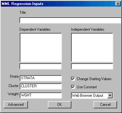
To run Regression left-click on the Statistics menu and select "MML Regression." The following dialogue box will open:

Specify the independent variables and the dependent variable. You may also elect to change the design variables, change the starting values, suppress the constant, and select the desired output format.
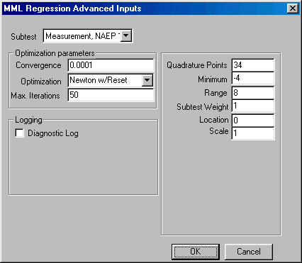
If you wish to change the default values of the program, click the Advanced button in the bottom left corner and the Advanced parameters dialogue box shown here will open:

You may now edit the values for quadrature points, minimum, range, subtest weight, convergence, maximum number of iterations allowed for convergence, and change the default optimization method. You may elect to create a diagnostic log.
When you are finished, click the OK button.
Click the OK button on the MML Regression dialogue box to begin the analysis.
Once the analysis is completed, you may perform either predicted values, posteriors, or t-tests on the results.
In NAEP, MML regression models are the models underlying plausible values. To obtain plausible values, NAEP estimates a large MML regression containing every background and contextual variable included in NAEP (known as conditioning variables), plus an additional random component. These marginal estimation procedures circumvent the need for calculating scores for individual students by providing consistent estimates of group or subgroup parameters.